Seven Detectors, One Small Dataset
It’s near the end of 2021. The city is vibrant again after COVID, and my best friend is coming for his birthday weekend. To celebrate, we go watch the Knicks play the Golden State Warriors. We have no idea we’ve bought tickets to history: Stephen Curry breaking Ray Allen’s all-time three-point record. My Knicks go on to lose, which is depressing, but we are in the building for this. As the ball drops through the net, Draymond Green is already cheering, Steph’s parents meet him on the court, and Ray Allen and Reggie Miller, the two retired players who held the record before him, are waiting to shake his hand. As a kid I spent years watching games with my father. This is the first time I’m there to witness history. As a huge basketball fan and computer vision engineer, I wonder: what can the computer see?
When Roboflow published How to Detect, Track, and Identify Basketball Players with Computer Vision, I obviously needed to grab the dataset and give it a try. This small dataset was a chance to work through the questions that come up every time you build a new object detector for your product team:
- How far can a finetuned model get on very little training data?
- Which model should we train? Is there actually a large difference between architectures, in accuracy or in speed?
- Permissive licenses are getting harder to come by, so do the restrictively licensed models actually perform better?
Two things came out of it. The top three models are a statistical tie, so accuracy does not pick a winner. License and latency do, and they point in opposite directions.
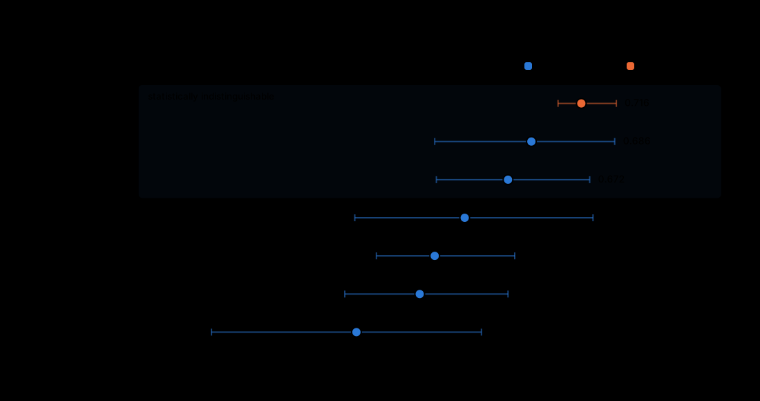 The whole result in one picture. Seven medium detectors at 640, with 95% intervals from a bootstrap that resamples the three test clips rather than the 94 correlated frames. The top three overlap. The rest of this post is how I got there and why those are the honest intervals.
All the code and results behind this post live at ortizeg/object-detection-eval.
Dataset
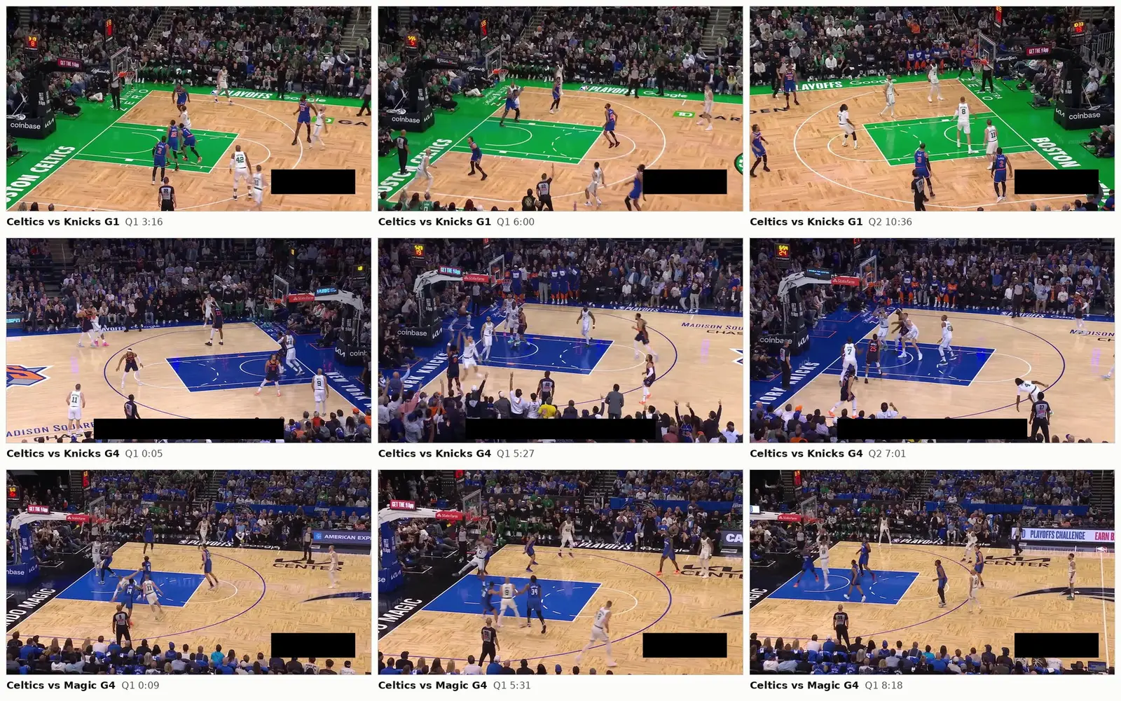 One frame from each of nine different clips. Rows are games: Celtics vs Knicks game 1 at TD Garden, Celtics vs Knicks game 4 at Madison Square Garden, Celtics vs Magic game 4 at the Kia Center. Broadcast angle, crowd, court color and lighting all shift between rows and barely shift within them. The black rectangle in the lower right of every frame is in the source export, not something I added.
Roboflow released a dataset with annotations for a basketball game including: player, referee, basketball ball, rim, ball in basket, jersey number, player in possession, player jump shot, player layup or dunk, and player shot block. The dataset is very small with a total of 654 images over the train (464), validation (96), and test (94) coming from 3 basketball games split into 21 clips, with no overlap of clips across train, validation, and test sets, though all three games appear in all three splits. The distribution of the labels across the set classes and sets are shown in the figure.
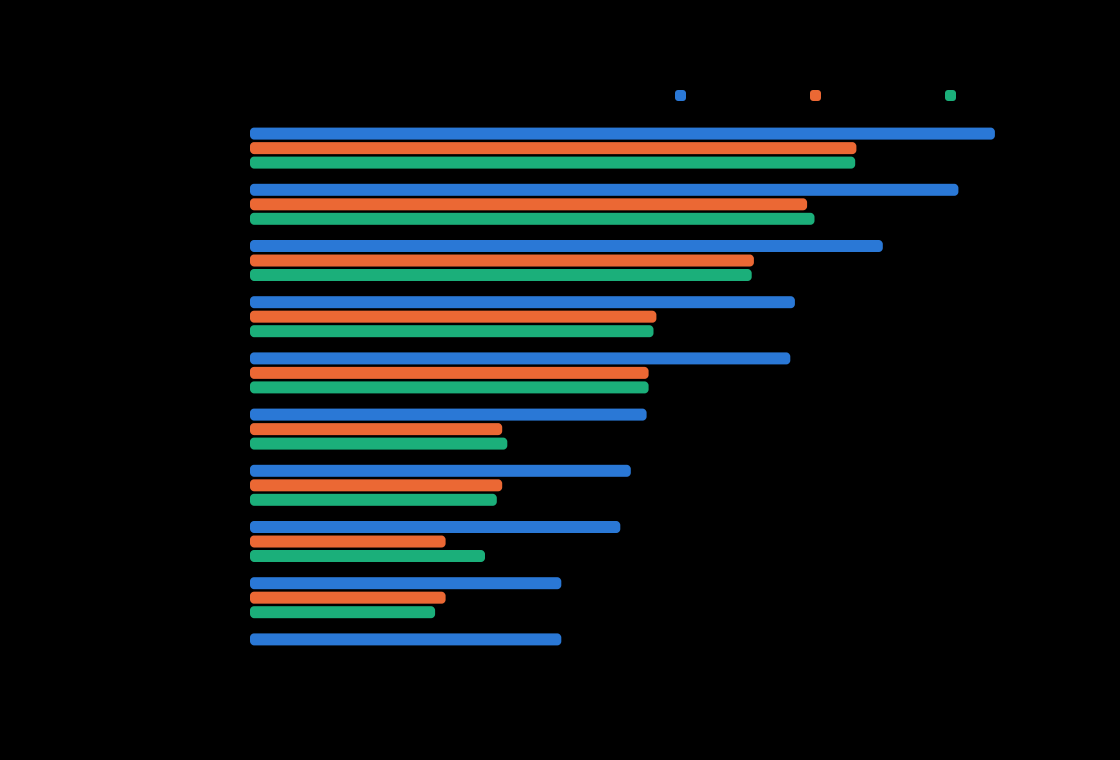 Counts are plotted on a log axis because
 player outnumbers player-layup-dunk by 185 to 1. Every bar carries its own count so nothing has to be read off the scale.
The difficulties of a dataset of this size are two fold:
- There are few samples in terms of quantity of frames, but also the samples are only from 3 basketball games, which limits generalization.
- The class distribution is heavily imbalanced, with 45% of samples belonging to the ‘player’ class alone, and the smallest classes only containing a maximum of ~1%.
The full breakdown of the dataset is in the table below:
| Class | Train | Valid | Test | Total | % of all boxes |
|---|---|---|---|---|---|
| player | 4,301 | 908 | 896 | 6,105 | 45.3% |
| number | 2,855 | 522 | 567 | 3,944 | 29.2% |
| referee | 1,221 | 287 | 280 | 1,788 | 13.3% |
| rim | 455 | 96 | 93 | 644 | 4.8% |
| ball | 432 | 88 | 88 | 608 | 4.5% |
| player-in-possession | 86 | 17 | 18 | 121 | 0.9% |
| player-jump-shot | 72 | 17 | 16 | 105 | 0.8% |
| player-shot-block | 64 | 9 | 14 | 87 | 0.6% |
| ball-in-basket | 33 | 9 | 8 | 50 | 0.4% |
| player-layup-dunk | 33 | 0 | 0 | 33 | 0.2% |
| Images | 464 | 96 | 94 | 654 | |
| Annotations | 9,552 | 1,953 | 1,980 | 13,485 | 100% |
I also report on a 5-class version, which folds the four player-* action states into player and ball-in-basket into ball. That is the taxonomy the zero-shot VLMs can be compared against, since they cannot reliably tell a jump shot from a shot block, or a ball in flight from a ball already through the net.
One more thing about this dataset that I did not appreciate until I went looking. The 654 images are not 654 independent photographs. They are 21 short playoff broadcast clips sampled at high frame rate, a mean of 31 frames each, and the test split is exactly 3 clips: 33 frames of Celtics vs Knicks game 4, 31 frames of Celtics vs Magic game 4, and 30 frames of Celtics vs Knicks game 1. Thirty frames spanning five seconds of one possession are near duplicates. Same players, same jerseys, same lighting, same camera pose. If a model nails one of them it will nail the other twenty-nine.
The splits are clip-disjoint, so no frame of a training clip shows up in test and there is no leakage of the severe kind. But all three splits draw from the same three games, so what the test set measures is generalization to unseen possessions inside known games, not to unseen arenas or unseen teams. Read every number below as an upper bound.
Mitigation paths for the class imbalance and the shortage of total samples are outside the coverage of this blog, but both inform the conclusions we make.
Models
Seven detectors, all at the medium tier, all trained and evaluated at input resolution 640x640. Medium-only is deliberate: comparing a small YOLO against a large DETR tells you about capacity, not architecture. The caveat is that “medium” by name spans 19M to 31M parameters, a 60% spread, so the roster is a comparison of architectures at their medium tier and not of models at identical capacity.
| Model | Released | Family | Backbone | Params | License |
|---|---|---|---|---|---|
| YOLOX-M | 2021 | YOLO / CNN | CSPDarknet | 25.3M | Apache-2.0 |
| RTMDet-M | 2022 | CNN (modern) | CSPNeXt | 27.3M | Apache-2.0 |
| DAMO-YOLO-M | 2022 | YOLO / CNN | TinyNAS-L35 | 28.0M | Apache-2.0 |
| DEIM-D-FINE-M | 2024 | DETR (real-time) | HGNetv2-B2 | 19.3M | Apache-2.0 |
| RT-DETRv2-M | 2024 | DETR (real-time) | ResNet-34-vd | 31.0M | Apache-2.0 |
| RF-DETR-M | 2025 | DETR (NAS) | DINOv2 windowed-small | 30.2M | Apache-2.0 |
| YOLO26m | 2026 | YOLO (NMS-free) | CSP-based | 20.4M | AGPL-3.0-only |
Here is a quick summary of what each adds for historical understanding.
| Model | The idea it adds |
|---|---|
| YOLOX-M | Anchors dropped, decoupled head, SimOTA dynamic label assignment. CSPDarknet, PAN neck, NMS at the end. |
| RTMDet-M | YOLOX with better parts: 5x5 depthwise convs, a head sharing weights but not BatchNorm across scales, soft label assignment. |
| DAMO-YOLO-M | The most engineered: TinyNAS-searched backbone, RepGFPN neck, near-empty head, AlignedOTA, distillation. |
| YOLO26m | Natively end-to-end. One-to-one matching emits 300 boxes with no NMS in the graph. Drops DFL, adds STAL to give small objects more positives. |
| RT-DETRv2-M | The DETR that first beat YOLOs in real time (RT-DETR): cheap intra-scale attention plus cross-scale CNN fusion, IoU-aware query selection. |
| DEIM-D-FINE-M | D-FINE predicts a distribution per box edge and sharpens it instead of regressing four numbers; DEIM raises positives per image. Both target DETR’s slow convergence. |
| RF-DETR-M | Built for small custom datasets: self-supervised DINOv2 backbone, decoder configuration found by NAS. |
Among the YOLO and CNN models the variable is how much engineering has gone in since 2021. YOLOX is the oldest and nothing about it is new. RTMDet and DAMO-YOLO are both explicit attempts to do it better, and DAMO’s published COCO figure at medium is 49.2 against YOLOX-M’s 47, though its official distilled weights are no longer downloadable, so I finetuned from the pre-distillation checkpoint at 48.7. YOLO26 is the newest, the only one here that is not Apache-2.0, and the one whose NMS-free head and STAL assignment are worth watching on a dataset whose hardest class is a basketball in flight. Its AGPL-3.0-only licensee gets its own section at the end.
Among the DETRs the variable is the backbone. They share a broadly similar decoder and differ most in what feeds it: plain ImageNet ResNet-34-vd for RT-DETRv2, HGNetv2 for DEIM, self-supervised DINOv2 for RF-DETR. RT-DETRv2 is the only model in the roster on a plain ImageNet backbone and it finishes last, though I ran no backbone swap and cannot separate that from the neck, head, assignment, augmentation and epoch budget that also vary. RF-DETR carries a caveat I owe it: DINOv2 is patch-14 with documented resolutions in multiples of 56, so 640 is off its native grid. The rfdetr library interpolates the position embeddings to fit, which is the intended path, but I never ran it at 560 or 672 for comparison. If any model here carries an untested handicap, it is that one.
Methodology
Training
All seven were finetuned on this dataset from their own COCO-pretrained checkpoints at 640x640, each on its own published training recipe. Seven recipes in seven environments is a versioning problem before it is a training one. Every model is configured with 11 output classes, matching the 11 category ids in the Roboflow export. These are basketball categories in COCO annotation format, not COCO’s own 80 classes. One of the eleven, basketball at id 0, carries zero annotations and is an artifact of the export, so only 10 ids ever appear in the data and the evaluated taxonomies are the 10-class raw set and the 5-class merge.
I deliberately did not run per-model learning rate or augmentation sweeps. Tuning effort is itself a source of unfairness: you tune hardest on the models you understand best, and then publish that as an architecture result. Architecture-specific hyperparameters stay at each model’s published default, and only the shared protocol is equalized.
That principle needed one exception, for genuine mechanical bugs. Two models ship warmup schedules tuned for COCO’s 117k images: DEIM and RT-DETRv2 both warm up over 2000 iterations, which on a 464-image training set is most of the run spent at a near-zero learning rate. DEIM’s first attempt produced mAP near zero for exactly this reason. Rescaling those warmups is fixing a mis-scaling, not tuning. RTMDet’s 1000-iteration warmup got the same scrutiny, and an ablation showed it was not a material handicap: native validation improved a point (0.542 to 0.552) while test 5-class moved 0.9 points the other way (0.628 to 0.619), well inside the interval. Its recipe default is what I report.
Metrics
Scoring is COCO-standard. The three numbers below differ only in how much box overlap they demand, and each asks a different question:
- mAP@50 (IoU 0.5): did the model find the object? Loose overlap counts. This is the detection question.
- mAP@75 (IoU 0.75): did it find the object and draw a tight box? This is the localization question.
- mAP@50:95: the average of AP at ten thresholds from 0.50 to 0.95 in steps of 0.05. This is the ranking metric, and it punishes sloppy boxes hard.
The gap between mAP@50 and mAP@75 is where a model tells on itself. A detector that scores 0.95 at IoU 0.5 and 0.64 at IoU 0.75 is seeing everything and localizing loosely.
Results
Overall accuracy
Five-class taxonomy, 94-image test split, sorted best to worst on the ranking metric:
| Model | mAP@50:95 | mAP@50 | mAP@75 |
|---|---|---|---|
| YOLO26m | 0.716 | 0.950 | 0.839 |
| DEIM-M | 0.686 | 0.942 | 0.788 |
| YOLOX-M | 0.672 | 0.934 | 0.787 |
| RF-DETR-M | 0.646 | 0.937 | 0.705 |
| RTMDet-M | 0.628 | 0.878 | 0.727 |
| DAMO-YOLO-M | 0.619 | 0.890 | 0.736 |
| RT-DETRv2-M | 0.581 | 0.862 | 0.637 |
Ten-class taxonomy, same models, same split, same protocol:
| Model | mAP@50:95 | mAP@50 | mAP@75 |
|---|---|---|---|
| DEIM-M | 0.643 | 0.857 | 0.745 |
| YOLO26m | 0.639 | 0.824 | 0.754 |
| RF-DETR-M | 0.592 | 0.812 | 0.657 |
| RTMDet-M | 0.580 | 0.778 | 0.677 |
| YOLOX-M | 0.580 | 0.789 | 0.688 |
| DAMO-YOLO-M | 0.541 | 0.788 | 0.671 |
| RT-DETRv2-M | 0.501 | 0.708 | 0.559 |
Two things jump out. First, every model drops 4 to 10 points going from 5 classes to 10, which is the rare action classes doing what 87 boxes of player-shot-block should be expected to do. Second, the top of the table reorders: DEIM-M edges ahead of YOLO26m by 0.003, and YOLOX-M falls from third to a tie for fourth.
Read that ordering with more caution than the 5-class one, since I cannot put an interval on it. The four sparse action classes carry 40% of the 10-class metric on 8, 14, 16 and 18 test boxes between them, and DEIM’s lead comes substantially from player-shot-block, where it beats YOLO26m by 0.35 AP on 14 boxes. I would not bet a deployment on 14 boxes, and neither should you. Treat this as a per-class breakdown that happens to be sorted, not as a second leaderboard.
One thing I did check: the 5-class merge relabels boxes without re-running NMS, so a duplicate could survive the collapse and flatter the DETRs. Suppressing those changes nothing, at most 0.0008 mAP@50:95 per model, ten times below the bootstrap’s own error.
That suppression came with a lesson about this domain, though. It only helps above IoU 0.9. At the usual 0.5 it makes every model worse, because two players standing shoulder to shoulder on a crowded court legitimately overlap that much, and suppressing one trades a false positive for a false negative. Only near-total overlap isolates a genuine artifact, which is the same box wearing two labels.
Every ranking claim here rests on a paired bootstrap: resample the test set with replacement, score every model on the same resampled set, take the difference within each replicate, repeat 1000 times, read the middle 95%. Pairing is what makes it work, because when a draw happens to be easy it is easy for everyone, so the shared difficulty term cancels in the subtraction. Run it resampling images and you assume 94 independent observations. Run it resampling clips, which is what the data actually is, and the intervals widen by 1.4x to 3.9x.
YOLO26m, DEIM-M and YOLOX-M are statistically indistinguishable. YOLO26m’s apparent 4.4 point lead over YOLOX-M carries a 95% interval of [-0.7, +7.4] points, which straddles zero. At the image level, 5 of the 6 adjacent pairs look significant. Once the resampling respects the clip structure, only 2 of 6 survive:
| Pair | Diff | Image-level CI | Clip-level CI | Verdict |
|---|---|---|---|---|
| YOLO26m vs DEIM-M | +0.029 | [+0.014, +0.044] | [-0.023, +0.075] | tie |
| DEIM-M vs YOLOX-M | +0.015 | [+0.004, +0.025] | [-0.001, +0.035] | tie |
| YOLOX-M vs RF-DETR-M | +0.025 | [+0.010, +0.041] | [-0.002, +0.049] | tie |
| RF-DETR-M vs RTMDet-M | +0.019 | [+0.003, +0.034] | [-0.012, +0.048] | tie |
| RTMDet-M vs DAMO-YOLO-M | +0.009 | [-0.002, +0.020] | [+0.003, +0.019] | significant |
| DAMO-YOLO-M vs RT-DETRv2-M | +0.038 | [+0.021, +0.053] | [+0.003, +0.081] | significant |
RTMDet vs DAMO-YOLO moves the other way for a reason. Its gap is small but consistent, with RTMDet edging DAMO-YOLO in all three clips, while the four pairs that collapse have differences that flip depending on which clip you score. Clustering rewards consistency and discounts raw magnitude. Note also that there is no multiple-comparison correction across the six tests, so at alpha 0.05 the family-wise false positive risk is around 26%.
Per-class accuracy
Five-class AP@50, with test-set support so you can see which columns to trust:
| Model | player (944) | ball (96) | referee (280) | rim (93) | number (567) |
|---|---|---|---|---|---|
| YOLO26m | 0.969 | 0.887 | 0.979 | 1.000 | 0.915 |
| DEIM-M | 0.987 | 0.836 | 0.995 | 1.000 | 0.891 |
| YOLOX-M | 0.980 | 0.784 | 0.989 | 1.000 | 0.917 |
| RF-DETR-M | 0.987 | 0.812 | 0.986 | 1.000 | 0.900 |
| RTMDet-M | 0.984 | 0.638 | 0.998 | 0.996 | 0.775 |
| DAMO-YOLO-M | 0.982 | 0.695 | 0.995 | 1.000 | 0.778 |
| RT-DETRv2-M | 0.976 | 0.499 | 0.948 | 1.000 | 0.887 |
Ten-class AP@50:
| Model | ball | ball-in-basket | number | player | in-possession | jump-shot | layup-dunk | shot-block | referee | rim |
|---|---|---|---|---|---|---|---|---|---|---|
| YOLO26m | 0.890 | 0.856 | 0.915 | 0.961 | 0.475 | 0.808 | — | 0.533 | 0.979 | 1.000 |
| DEIM-M | 0.851 | 0.718 | 0.892 | 0.975 | 0.455 | 0.942 | — | 0.886 | 0.995 | 1.000 |
| YOLOX-M | 0.789 | 0.734 | 0.910 | 0.939 | 0.410 | 0.785 | — | 0.544 | 0.989 | 1.000 |
| RF-DETR-M | 0.819 | 0.720 | 0.899 | 0.982 | 0.640 | 0.731 | — | 0.530 | 0.987 | 1.000 |
| RTMDet-M | 0.651 | 0.404 | 0.775 | 0.981 | 0.553 | 0.930 | — | 0.718 | 0.998 | 0.996 |
| DAMO-YOLO-M | 0.708 | 0.636 | 0.779 | 0.977 | 0.468 | 0.771 | — | 0.762 | 0.995 | 1.000 |
| RT-DETRv2-M | 0.531 | 0.327 | 0.887 | 0.955 | 0.089 | 0.818 | — | 0.817 | 0.948 | 1.000 |
The em dash in the player-layup-dunk column is not a formatting slip and it is not 0.000. That class has zero test support, so its AP is undefined. A present-but-zero class would render 0.000. The report generator distinguishes the two on purpose, because “the model completely failed at dunks” and “we have no dunks to score against” are very different sentences.
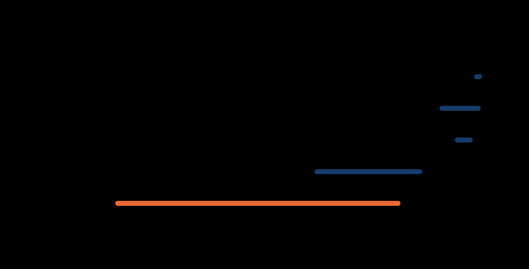 The span between the worst and best model on each class, at IoU 0.5. Three of the five are effectively solved by everyone. Note this is AP@50; the ranking metric is mAP@50:95 and tells a different story.
Read the five-class table by column and at IoU 0.5 the task is close to solved for everyone. player spans 0.969 to 0.987 across seven architectures. referee spans 0.948 to 0.998. rim is 0.996 to 1.000, effectively saturated, because a rim is large, static, high contrast and bolted to the same spot in every frame. ball spans 0.499 to 0.887, a 39 point gap, with jersey number a distant second at 14 points. Those two are the only classes where finding the object is still hard.
I was ready to write that the ball therefore drives the leaderboard, and the tables would not let me. That per-class table is AP@50; the ranking metric is mAP@50:95, and I do not compute per-class AP@50:95, so the jump from one to the other is not mine to make. It also fails on a case sitting in my own numbers: RF-DETR-M beats YOLOX-M on ball (0.812 vs 0.784) and on overall mAP@50 (0.937 vs 0.934), and still loses mAP@50:95 by 2.6 points. The column that separates them is mAP@75, 0.705 against 0.787. There is a second reversal, DAMO-YOLO over RTMDet, that runs on something else entirely and that I cannot resolve from the columns I publish.
So the honest reading is less about the ball and more about box tightness. Once everything finds the objects, the leaderboard is largely a localization ranking, and RF-DETR against YOLOX is the pair where every published number lines up behind that: a find-everything, box-it-loosely model losing to a tighter one. That matters more than a class ranking, because loose boxes are cheap in an analytics pipeline and expensive in anything that crops.
Whatever separates models on ball, it is not the head paradigm. DEIM (0.836) and RF-DETR (0.812) read it far better than RT-DETRv2 (0.499) while all three are DETRs decoding in-graph, so the split runs straight through one architecture family. The tempting story is the backbone, HGNetv2 and DINOv2 against a plain R34-vd in exactly that order, and I cannot support it for the reasons above. YOLO26m leads outright at 0.887, which is what STAL is supposed to buy you.
Latency, and the benchmark that lied to me
TensorRT fp16, batch 1, measured to final boxes so every model reports the same endpoint (the three dense-head graphs, YOLOX, DAMO-YOLO and RTMDet, get an EfficientNMS_TRT plugin grafted on; YOLO26m and the DETRs already produce final boxes in-graph):
| Model | Median (ms) | P99 (ms) | FPS | License |
|---|---|---|---|---|
| YOLOX-M | 5.68 | 5.83 | 176 | Apache-2.0 |
| YOLO26m | 5.85 | 6.00 | 171 | AGPL-3.0-only |
| DEIM-M | 6.61 | 7.16 | 151 | Apache-2.0 |
| DAMO-YOLO-M | 6.70 | 6.83 | 149 | Apache-2.0 |
| RF-DETR-M | 7.71 | 7.91 | 130 | Apache-2.0 |
| RT-DETRv2-M | 7.93 | 8.10 | 126 | Apache-2.0 |
| RTMDet-M | 8.19 | 8.54 | 122 | Apache-2.0 |
 The entire roster lives in a 2.5 ms band. All three dense-head models are grafted at the same conf 0.01, so every horizontal position is a matched measurement.
The whole field fits inside 5.7 to 8.2 ms, so on a T4 the architecture choice barely moves latency and the accuracy question, such as it is, matters more.
The gaps at the top are small enough to keep in perspective. YOLOX-M’s 5.68 and YOLO26m’s 5.85 are 0.17 ms apart. The ordering is at least consistent, since YOLOX-M’s p99 (5.83) sits just under YOLO26m’s median, but a fifth of a millisecond is not a reason to pick a model. What the table clearly supports is that both are about a millisecond clear of the DETRs.
The second thing is where the milliseconds actually go. All three dense heads are grafted at the same conf 0.01, and at that matched threshold the NMS cost is wildly uneven. YOLOX-M’s is free, its grafted engine landing within noise of its raw 5.76 ms model-only build, while DAMO-YOLO-M’s costs +1.49 ms, taking it from 5.21 ms to 6.70. And 5.21 ms is worth pausing on: stripped of NMS, DAMO-YOLO-M has the fastest network in the roster, ahead of YOLOX-M. What separates them at the same threshold is how many candidate boxes each head throws at NMS, and DAMO’s head floods it. RTMDet’s ungrafted graph will not build under TensorRT at all, so its delta stays unmeasurable. One more thing survives: YOLO26m’s NMS-free head buys nothing on GPU, since at 5.85 ms it still trails YOLOX-M with NMS included.
Where NMS-free pays off is CPU, and even there the benefit is narrower than the pitch suggests. These numbers come from a short-lived single-tenant GCP n2-standard-8, CPU-only, with the machine spec and ONNX Runtime version recorded alongside the results. Dropping the confidence threshold from 0.25 to 0.01 costs DAMO-YOLO +131.9 ms of Python NMS, taking it from 169 ms to 301, because its head floods the sort loop with low-score boxes. Every other model in the roster lands within 8.1 ms, which at this scale is noise: YOLOX +1.1, RT-DETRv2 +2.4, YOLO26m +2.6, DEIM +5.6, RTMDet +7.7, RF-DETR +8.1. So the edge advantage is real and it belongs to one model’s head design, not to NMS-free architectures as a class.
Those absolutes, 170 to 380 ms, are 25 to 50 times the fp16 GPU numbers, which is the expected gap for a no-accelerator baseline. The re-measurement is worth a paragraph for a different reason: the contention failure mode described at the end of this section showed up again, on CPU this time. The first conf=0.01 pass read almost every model 85 to 96% slower than an immediate rerun, including architecturally NMS-free models that have no reason to care about a confidence threshold. That physical impossibility is what gave it away. A same-config stability check caught it, the run was discarded, and a third pass confirmed the numbers above. Getting burned once taught me to build the check. The check is what makes the second set of numbers worth printing.
I also have to report an embarrassment here, because it is the most useful thing in this section. My first latency run was on a shared vast.ai T4, and it was wrong in a way that produced a published conclusion. It read DEIM-M at 43.00 ms against its true 6.61, and it inverted the speed ranking, putting RF-DETR first and YOLOX fifth when the honest order is close to the reverse. Re-measuring byte-identical ONNX under the same TensorRT 10.3.0 on a sole-tenant instance with persistence mode on and the SM clock locked recovered the band for four of the seven and brought the other three within about a millisecond of it, with a residual I still cannot explain. Same hardware model, same engine, same graph. The only variable was the neighbors. Benchmark on a dedicated instance with locked clocks, or do not report latency.
What this actually means for picking a model
Accuracy does not separate the top three, so the choice gets made on the two axes that do.
| mAP@50:95 | fp16 to-boxes | License | |
|---|---|---|---|
| YOLOX-M | 0.672 | 5.68 ms | Apache-2.0 |
| YOLO26m | 0.716 | 5.85 ms | AGPL-3.0-only |
| DEIM-M | 0.686 | 6.61 ms | Apache-2.0 |
YOLO26m has the best point estimate and the license I cannot ship. AGPL-3.0-only means commercial serving needs a paid Ultralytics license or an open-sourced inference stack, and Ultralytics’ stated position is that weights finetuned with their code are derivative works, so a model trained on your own proprietary footage may be encumbered. That reading is contested and I am not a lawyer, but it is a diligence risk with a price tag. It is also not hypothetical: YOLO26m is the one row in this comparison whose weights I cannot redistribute, which makes it the one row a reader cannot fully reproduce from my repo.
So: YOLOX-M is the defensible default. Take DEIM-M if you want the best permissive point estimate and can afford one more millisecond, and YOLO26m only if the license genuinely is not a constraint for you.
One caveat, if the target is a phone or an NPU
Everything above is a server-GPU story, where the top three sit within a millisecond of each other. On mobile silicon the question is whether the model converts at all, and the two families are far apart.
The DETRs here barely leave the server. DEIM and D-FINE ship an ONNX exporter and little else: no CoreML, no TFLite, no Qualcomm path in the repo. The DETRs that do reach Qualcomm’s AI Hub are float-only, with their quantized and TFLite paths disabled for accuracy failures. The conv detectors are the opposite: YOLOX and YOLO26 carry the full int8 ladder and export to the mobile runtimes you would target.
I have not run any of these on a device myself. Everything in this section is read off vendor manifests and export scripts, which is the weakest evidence in the post, and I am flagging it as such rather than dressing it up. What I would do before committing is export one candidate to the actual target and measure it.
So if you are shipping to iOS, Android or a Hexagon NPU, this lands harder on YOLOX-M than the licensing argument does, and the price is small and specific. Against DEIM-M you give up 5.2 points of ball AP@50 (0.784 vs 0.836) and take 2.6 back on jersey number (0.917 vs 0.891). Player, referee and rim are saturated either way. The whole edge decision reduces to one question: is the basketball itself worth five points to your product.
What I did not control for
Four things that change how much weight this leaderboard can carry, collected here rather than scattered through the methodology.
Training-seed variance is unmeasured, and it is probably the biggest one. The bootstrap resamples the test set; the weights are frozen. On 464 training images, run-to-run seed variance is plausibly larger than the sampling uncertainty I do quantify, and I did not measure it.
Checkpoint selection was not equalized. Every model’s checkpoint was chosen by best score on a 96-image, 3-clip validation set, and the number of candidate checkpoints differed by roughly ten times across the roster, since some recipes evaluate every epoch and others every tenth. That is an optimistic bias, and it is unequal across these seven.
Three clusters cannot give a calibrated interval. Ten distinct resamples means any 95% label is coarser than two decimals suggest, however exact the arithmetic. Read “significant” as “the sign held in every clip I have,” the strongest statement three clips support, and not as a hypothesis test.
The scorer carries a known offset the size of my top gaps. YOLOX-S reads 39.6 against 40.5 published, the supervision versus pycocotools gap. That is 0.9 points, measured on one dense head with NMS. Whether it holds for a 300-query DETR emitting dense low-confidence boxes I do not know, and there is no reason to assume it does.
None of these change the shape of the result.
Conclusions
I opened with three questions. Here is where I landed on each, plus one I did not ask.
How far does a finetuned model get on very little data? Further than it has any right to. 464 training images from three games produced detectors at 0.72 mAP@50:95 on the five-class task, with player, referee and rim effectively solved by every model in the roster. If your classes are visually distinct and your domain is narrow, a few hundred labeled frames is a working product. What that number does not buy is generalization. Every split here shares the same three games, so this is performance on unseen possessions in known arenas, and a fourth game would cost you something I cannot quantify. When there is no fourth game to label, generating one is the other lever: on a redaction detector synthetic frames ended up supplying 30% of the training data.
Is there a large difference between architectures? Not on accuracy. Once the test set’s three-clip structure is respected, YOLO26m, DEIM-M and YOLOX-M cannot be separated. Architecture family is not destiny either: the YOLO and CNN group holds first, third, fifth and sixth, the DETR group holds second, fourth and last. The one class that still separates anything is ball, spanning 0.499 to 0.887 AP@50, and even there the ranking metric turns out to be measuring box tightness more than detection. On latency the whole roster fits inside 2.5 ms on a T4, which is to say the architecture choice barely moves it.
Do the restrictively licensed models actually work better? On this dataset, no. YOLO26m posts the best point estimate and it is the one model I cannot ship without a paid license or an open-sourced stack. The best permissive model gives up no measurable accuracy to it. YOLOX-M is a 2021 architecture, it is the fastest thing I measured at a matched threshold, it is Apache-2.0 end to end, and it is statistically tied with the newest model on the board. If you are shipping to a phone or an NPU that gap widens further in its favor, because the DETRs barely convert.
There is a fourth question I have not answered here: how far a generic zero-shot detector gets you before you train anything at all. Zero-shot classification held up better than I expected the last time I pointed it at video; whether detection does is the next post.
Resources
Code and data
- Evaluation harness, reports, and all committed results: ortizeg/object-detection-eval (published docs)
- Finetuned weights (8 of 10 models, SHA-256 verified, Apache-2.0): huggingface.co/ortizeg
- Dataset, the exact export used here: ego-playground/basketball-player-detection-3 v1, CC BY 4.0
- The blog that started this: How to Detect, Track, and Identify Basketball Players with Computer Vision
Papers
- YOLOX: Exceeding YOLO Series in 2021 (code)
- RTMDet: An Empirical Study of Designing Real-Time Object Detectors (code)
- DAMO-YOLO: A Report on Real-Time Object Detection Design (code)
- YOLO26: Ultralytics documentation (code)
- RT-DETR: DETRs Beat YOLOs on Real-time Object Detection, CVPR 2024
- RT-DETRv2: Improved Baseline with Bag-of-Freebies (code)
- D-FINE: Redefine Regression Task in DETRs as Fine-grained Distribution Refinement, ICLR 2025 (code)
- DEIM: DETR with Improved Matching for Fast Convergence, CVPR 2025 (code)
- RF-DETR: Neural Architecture Search for Real-Time Detection Transformers, ICLR 2026 (code)
- DINOv2: Learning Robust Visual Features without Supervision
Tools
- supervision for mAP scoring, pinned at 0.29.1
- ONNX Runtime and TensorRT for the latency work
- onnx-graphsurgeon for grafting
EfficientNMS_TRTonto the dense heads
Further reading on edge and mobile deployment
- Qualcomm AI Hub model zoo: per-model
manifest.yamlandperf.yamlcarry each model’s runtime status, disabled paths and supported precisions (D-FINE, RF-DETR, YOLOX, Deformable-DETR) - Qualcomm AI Engine Direct supported ONNX ops:
GridSampleis supported, 4D and 5D inputs only - coremltools
grid_samplerto MILresample, plus the Apple developer forum reports thatresampleruns CPU-only with no GPU path - RF-DETR’s TFLite converter: the clearest write-up anywhere of how
GridSamplesilently breaks under TFLite, and the gather rewrite that fixes it - RT-DETRv2 discrete-sampling checkpoints:
grid_sampleswapped forindex_selectat 0.1 to 0.4 AP50